Visualization Theory
Inner Product, Norm, and Angle
Fixing some \(d\) and \(M\), we can define the inner product of two tensors by
where \(\bar{U}\) indicates complex conjugate, if appropriate. If \(T\) and \(U\) are represented with separation ranks \(r\) and \(s\) using vectors \(V^l_k\) and \(W^l_k\), then their inner product can also be computed via
which costs \(\mathcal{O}(rsdM)\) operations.
With this inner product we can define length with the norm
We can also define the angle between \(T\) and \(U\) relative to the origin with
realizing that this may be a complex number if \(T\) or \(U\) is complex.
The operations necessary for the visualization will be based on this inner product, and so are essentially coordinate-free. In particular, a separable change of coordinates does not effect the vizualization.
Intersections
We now consider how to visualize a set \(S\) of tensors. Since \(S\) is defined as a subset of \(R^{M^d}\) we cannot visualize it all at once. Instead we can intersect it with a simpler object and visualize this intersection. Any two distinct tensors \(T_1\) and \(T_2\) define a line, which can be represented by
Similarly, any three tensors \(T_1\), \(T_2\), and \(T_2\) that do not lie on a line define a plane
By intersecting \(S\) with one of these simpler objects we obtain something that we can visualize.
Including Nearby Points
Unfortunately, in practice the straightforward intersection described above yields too few points to plot. If we proceed by generating points in \(S\), the probability that any of them lie in the given line/plane is virtually zero. If we proceed by generating points in the line/plane then we need to test their membership in \(S\). For the sets we are interested in this membership test can fail, and at best can produce a tensor in \(S\) within some small distance of the tensor we are checking.
A star-shaped set is a set \(S\) such that \(T\in S \Rightarrow cT \in S\) for any scalar \(c\). Such a \(S\) is connected and simply connected. Instead of asking if \(T\in S\) is on our plotting line/plane, we can ask if \(cT\) is on our plotting line/plane for some \(c\), and if so, plot that \(cT\). Thus we can increase the number of plotted points and remove the uninteresting scalar structure. Formally, we consider tensors that are positive scalar multiples of one another to be equivalent. Locally, this is similar to restricting to tensors of norm one. (Identifying negative scalar multiples as well does not seem to be worthwhile.)
We will add further information to the visualization by including points that are in \(S\) but not on the plotting line/plane and coloring them to indicate how far from the plotting plane they are. Since we identify \(T\) and \(cT\) we measure “how far” using an angle instead of a distance.
We will describe the the case for a plane, since the case for a line is a simple modification of it. From the three points \(T_1\), \(T_2\), and \(T_3\) that define our plane, we define the matrix
Given \(T\in S\), its projection onto the span of \(T_1\), \(T_2\), and \(T_3\) is given by
with
Dividing by the scalar \(c_1+c_2+c_3\), we obtain the tensor
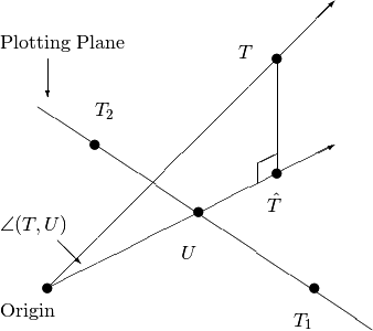
which lies on the plotting plane. To measure how much \(T\) failed to be on the plane, we compute the angle
An angle of zero indicates that some scalar multiple of \(T\) is on the plane and an angle of \(\pi/2\) indicates that \(T\) is orthogonal to the span of \(T_1\), \(T_2\), and \(T_3\). This projection process (neglecting \(T_3\)) is illustrated below:
To indicate this angle in the visualization, we color the plotted point with black indicting angle nearly zero, then through a spectrum of ever-lightening colors until light yellow indicates angles near \(\pi/2\). We use the colors
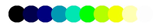
and bin the angles logarithmicly by
In cases where more than one tensor projects to the same plotting point, we plot the darker of the two. Since we plot points as small discs, in cases where the discs overlap we plot the darker disc on top.
If \(T\) is orthogonal to the span of \(T_1\), \(T_2\), and \(T_3\) we will have \(c_1=c_2=c_3=0\) and cannot consruct \(U\). Thus \(T\) should not appear in the visualization. (Numerically one produces a white point at a location determined by roundoff errors.)
Real Tensors, plotted on a real plane
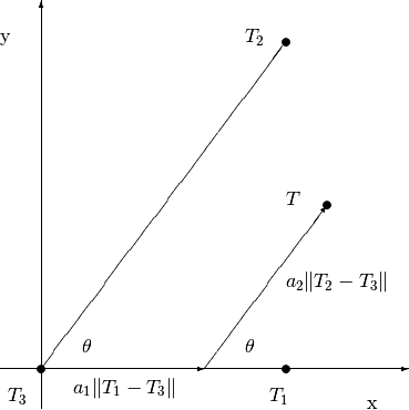
For tensors over the real numbers, our tool uses three tensors yielding a plane, so we now consider that case in more detail. We arbitrarily choose to orient the visualization so that \(T_3\) is at \((0,0)\) and \(T_1\) is in the direction \((1,0)\). The angle from \(T_1\) to \(T_3\) to \(T_2\) is given by
so \(T_2\) is in the direction \((\cos(\theta),\sin(\theta))\). A tensor \(T=a_1 T_1+a_2T_2+(1-a_1-a_2)T_3\) is at the point
This plotting geometry is illustrated below:
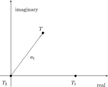
Complex Tensors, plotted on a complex line
For tensors over the complex numbers, our tool uses two tensors yielding a complex line. We arbitrarily choose to orient the visualization so that \(T_2\) is at \(0+0i\) and \(T_1\) is in the direction \(1+0i\). A tensor \(T=a_1 T_1+(1-a_1)T_2\) is at the complex point \(a_1\). This plotting geometry is illustrated below: